Abstract
In this exercise, we explore different initialization, optimization and regularization techniques and model a multi-classification problem using Python and Tensorflow incorporatig some of these techniques.
Credits: Coursera Deep Learning Specialization
Optimization Methods
1 - (Batch) Gradient Descent
A simple optimization method in machine learning is gradient descent (GD). When you take gradient steps with respect to all $m$ examples on each step, it is also called Batch Gradient Descent. The gradient descent rule is, for $l = 1, …, L$:
\[W^{[l]} = W^{[l]} - \alpha \text{ } dW^{[l]} \tag{1}\] \[b^{[l]} = b^{[l]} - \alpha \text{ } db^{[l]} \tag{2}\]where L is the number of layers and $\alpha$ is the learning rate.
X = data_input
Y = labels
m = X.shape[1]  # Number of training examples
parameters = initialize_parameters(layers_dims)
for i in range(0, num_iterations):
    # Forward propagation
    a, caches = forward_propagation(X, parameters)
    # Compute cost
    cost_total = compute_cost(a, Y)  # Cost for m training examples
    # Backward propagation
    grads = backward_propagation(a, caches, parameters)
    # Update parameters
    parameters = update_parameters(parameters, grads)
    # Compute average cost
    cost_avg = cost_total / m
2 - Stocastic Gradient Descent
A variant of Gradient Descent is Stochastic Gradient Descent (SGD), which is equivalent to mini-batch gradient descent, where each mini-batch has just 1 example. What changes is that you would be computing gradients on just one training example at a time, rather than on the whole training set. The code examples below illustrate the difference between stochastic gradient descent and (batch) gradient descent.
X = data_input
Y = labels
m = X.shape[1]  # Number of training examples
parameters = initialize_parameters(layers_dims)
for i in range(0, num_iterations):
    cost_total = 0
    for j in range(0, m):
        # Forward propagation
        a, caches = forward_propagation(X[:,j], parameters)
        # Compute cost
        cost_total += compute_cost(a, Y[:,j])  # Cost for one training example
        # Backward propagation
        grads = backward_propagation(a, caches, parameters)
        # Update parameters
        parameters = update_parameters(parameters, grads)
    # Compute average cost
    cost_avg = cost_total / m
In Stochastic Gradient Descent, you use only 1 training example before updating the gradients. When the training set is large, SGD can be faster. But the parameters will “oscillate” toward the minimum rather than converge smoothly. Here’s what that looks like:

"+" denotes a minimum of the cost. SGD leads to many oscillations to reach convergence, but each step is a lot faster to compute for SGD than it is for GD, as it uses only one training example (vs. the whole batch for GD).
Implementing SGD requires 3 for-loops in total:
- Over the number of iterations
- Over the $m$ training examples
- Over the layers (to update all parameters, from $(W^{[1]},b^{[1]})$ to $(W^{[L]},b^{[L]})$ )
In practice, you’ll often get faster results if you don’t use the entire training set, or just one training example, to perform each update.
3 - Mini-Batch Gradient Descent
Mini-batch gradient descent uses an intermediate number of examples for each step. With mini-batch gradient descent, you loop over the mini-batches instead of looping over individual training examples.
X = data_input
Y = labels
m = X.shape[1]  # Number of training examples
parameters = initialize_parameters(layers_dims)
for i in range(0, num_epochs):
    #generate mini batches by shuffling and partitioning
    minibatches = random_mini_batches(X, Y, mini_batch_size)
    cost_total = 0
    for minibatch in minibatches:
        #get x and y component of each minibatch
        (mini_X, mini_Y) = minibatch
        # Forward propagation
        a, caches = forward_propagation(mini_X, parameters)
        # Compute cost
        cost_total += compute_cost(a, mini_Y)  # Cost for one training example
        # Backward propagation
        grads = backward_propagation(a, mini_Y, caches)
        # Update parameters
        parameters = update_parameters(parameters, grads, learning_rate)
    # Compute average cost
    cost_avg = cost_total / m

"+" denotes a minimum of the cost. Using mini-batches in your optimization algorithm often leads to faster optimization.
There are two steps:
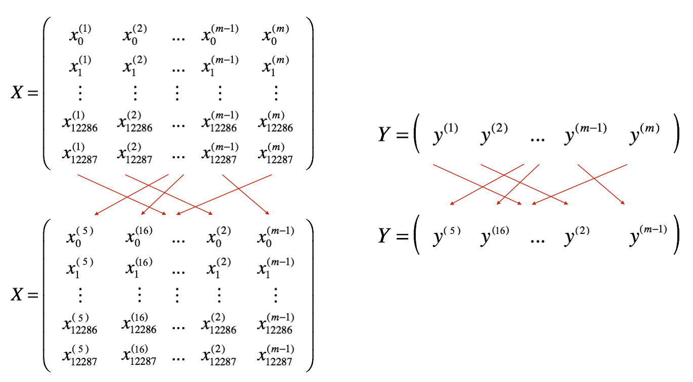
- Shuffle: Create a shuffled version of the training set (X, Y) as shown below. Each column of X and Y represents a training example. Note that the random shuffling is done synchronously between X and Y. Such that after the shuffling the $i^{th}$ column of X is the example corresponding to the $i^{th}$ label in Y. The shuffling step ensures that examples will be split randomly into different mini-batches.
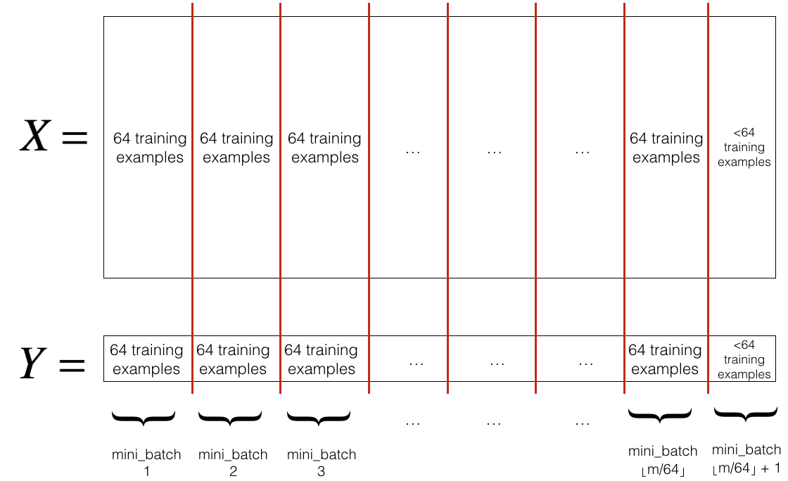
- Partition: Partition the shuffled (X, Y) into mini-batches of size
mini_batch_size(here 64). Note that the number of training examples is not always divisible bymini_batch_size. The last mini batch might be smaller. When the final mini-batch is smaller than the fullmini_batch_size, it will look like this:
- Shuffling and Partitioning are the two steps required to build mini-batches
- Powers of two are often chosen to be the mini-batch size, e.g., 16, 32, 64, 128.
4 - Momentum
Because mini-batch gradient descent makes a parameter update after seeing just a subset of examples, the direction of the update has some variance, and so the path taken by mini-batch gradient descent will “oscillate” toward convergence. Using momentum can reduce these oscillations.
Momentum takes into account the past gradients to smooth out the update. The ‘direction’ of the previous gradients is stored in the variable $v$. Formally, this will be the exponentially weighted average of the gradient on previous steps. You can also think of $v$ as the “velocity” of a ball rolling downhill, building up speed (and momentum) according to the direction of the gradient/slope of the hill.
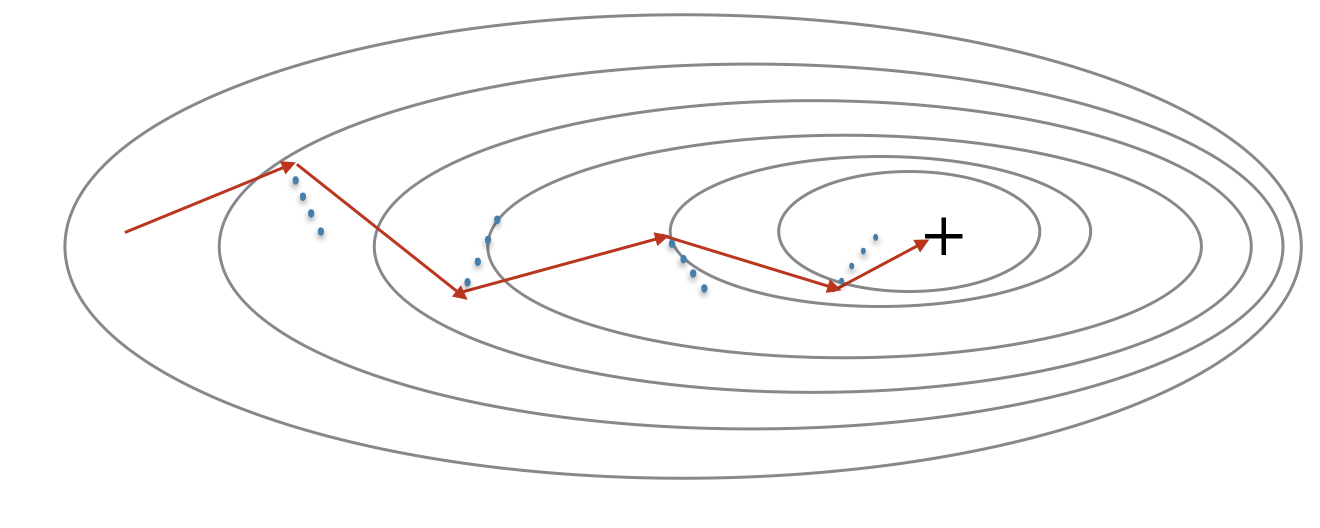
"+" denotes a minimum of the cost. Using mini-batches in your optimization algorithm often leads to faster optimization. The red arrows show the direction taken by one step of mini-batch gradient descent with momentum. The blue points show the direction of the gradient (with respect to the current mini-batch) on each step. Rather than just following the gradient, the gradient is allowed to influence v and then take a step in the direction of v.
The velocity, $v$, is a python dictionary that needs to be initialized with arrays of zeros. Its keys are the same as those in the grads dictionary, that is:
for $l =1,…,L$:
v["dW" + str(l)] = ... #(numpy array of zeros with the same shape as parameters["W" + str(l)])
v["db" + str(l)] = ... #(numpy array of zeros with the same shape as parameters["b" + str(l)])
Now, implement the parameters update with momentum. The momentum update rule is, for $l = 1, …, L$:
\[\begin{cases} v_{dW^{[l]}} = \beta v_{dW^{[l]}} + (1 - \beta) dW^{[l]} \\ W^{[l]} = W^{[l]} - \alpha v_{dW^{[l]}} \end{cases}\tag{3}\] \[\begin{cases} v_{db^{[l]}} = \beta v_{db^{[l]}} + (1 - \beta) db^{[l]} \\ b^{[l]} = b^{[l]} - \alpha v_{db^{[l]}} \end{cases}\tag{4}\]where L is the number of layers, $\beta$ is the momentum and $\alpha$ is the learning rate.
- The velocity is initialized with zeros. So the algorithm will take a few iterations to “build up” velocity and start to take bigger steps.
- If $\beta = 0$, then this just becomes standard gradient descent without momentum.
- The larger the momentum $\beta$ is, the smoother the update, because it takes the past gradients into account more. But if $\beta$ is too big, it could also smooth out the updates too much.
- Common values for $\beta$ range from 0.8 to 0.999. If you don’t feel inclined to tune this, $\beta = 0.9$ is often a reasonable default.
- Tuning the optimal $\beta$ for your model might require trying several values to see what works best in terms of reducing the value of the cost function $J$.
- Momentum takes past gradients into account to smooth out the steps of gradient descent. It can be applied with batch gradient descent, mini-batch gradient descent or stochastic gradient descent.
- You have to tune a momentum hyperparameter $\beta$ and a learning rate $\alpha$.
5 - Adam Optimizer
Adam is one of the most effective optimization algorithms for training neural networks. It combines ideas from RMSProp and Momentum.
How does Adam work?
- It calculates an exponentially weighted average of past gradients, and stores it in variables $v$ (before bias correction) and $v^{corrected}$ (with bias correction).
- It calculates an exponentially weighted average of the squares of the past gradients, and stores it in variables $s$ (before bias correction) and $s^{corrected}$ (with bias correction).
- It updates parameters in a direction based on combining information from “1” and “2”.
The update rule is, for $l = 1, …, L$:
\[\begin{cases} v_{dW^{[l]}} = \beta_1 v_{dW^{[l]}} + (1 - \beta_1) \frac{\partial \mathcal{J} }{ \partial W^{[l]} } \\ v^{corrected}_{dW^{[l]}} = \frac{v_{dW^{[l]}}}{1 - (\beta_1)^t} \\ s_{dW^{[l]}} = \beta_2 s_{dW^{[l]}} + (1 - \beta_2) (\frac{\partial \mathcal{J} }{\partial W^{[l]} })^2 \\ s^{corrected}_{dW^{[l]}} = \frac{s_{dW^{[l]}}}{1 - (\beta_2)^t} \\ W^{[l]} = W^{[l]} - \alpha \frac{v^{corrected}_{dW^{[l]}}}{\sqrt{s^{corrected}_{dW^{[l]}}} + \varepsilon} \end{cases}\]where:
- t counts the number of steps taken of Adam
- L is the number of layers
- $\beta_1$ and $\beta_2$ are hyperparameters that control the two exponentially weighted averages.
- $\alpha$ is the learning rate
- $\varepsilon$ is a very small number to avoid dividing by zero
Initialize the Adam variables $v, s$ which keep track of the past information.The variables $v, s$ are python dictionaries that need to be initialized with arrays of zeros. Their keys are the same as for grads, that is:
for $l = 1, …, L$:
v["dW" + str(l)] = ... #(numpy array of zeros with the same shape as parameters["W" + str(l)])
v["db" + str(l)] = ... #(numpy array of zeros with the same shape as parameters["b" + str(l)])
s["dW" + str(l)] = ... #(numpy array of zeros with the same shape as parameters["W" + str(l)])
s["db" + str(l)] = ... #(numpy array of zeros with the same shape as parameters["b" + str(l)])
Initialization
In general, initializing all the weights to zero results in the network failing to break symmetry. This means that every neuron in each layer will learn the same thing, so you might as well be training a neural network with $n^{[l]}=1$ for every layer. This way, the network is no more powerful than a linear classifier like logistic regression. The weights $W^{[l]}$ should be initialized randomly to small values to break symmetry. Initializing weights to very large random values doesn’t work well. However, it’s okay to initialize the biases $b^{[l]}$ to zeros. Symmetry is still broken so long as $W^{[l]}$ is initialized randomly. We usually initialize weights as np.random.randn(..,..) * 0.01. For ReLU activation, we usually use “He initialization” which is similar to “Xavier Initialization” except Xavier initialization uses a scaling factor for the weights $W^{[l]}$ of sqrt(1./layers_dims[l-1]) whereas “He initialization” would use sqrt(2./layers_dims[l-1]). Different initializations lead to very different results.
1 - Random Initialization:
Here is the implementation for $L=1$ (one layer neural network). This is initializing parameters randomly.
if L == 1:
    parameters["W" + str(L)] = np.random.randn(layer_dims[1], layer_dims[0]) * 0.01
    parameters["b" + str(L)] = np.zeros((layer_dims[1], 1))
- The weights $W^{[l]}$ should be initialized randomly to break symmetry.
- However, it’s okay to initialize the biases $b^{[l]}$ to zeros. Symmetry is still broken so long as $W^{[l]}$ is initialized randomly. To break symmetry, initialize the weights randomly. Following random initialization, each neuron can then proceed to learn a different function of its inputs
- Initializing weights to very large random values doesn’t work well.
- Initializing with small random values should do better.
- When used for weight initialization, randn() helps most the weights to Avoid being close to the extremes, allocating most of them in the center of the range.
2 - He Initialization:
- This is named for the first author of He et al., 2015. (If you have heard of “Xavier initialization”, this is similar except Xavier initialization uses a scaling factor for the weights $W^{[l]}$ of
sqrt(1./layers_dims[l-1])where He initialization would usesqrt(2./layers_dims[l-1]).) - You will multiply it by $\sqrt{\frac{2}{\text{dimension of the previous layer}}}$, which is what He initialization recommends for layers with a ReLU activation.
Regularization
If the regularization becomes very large, then dw is very large, the parameters W becomes very small, so Z will be relatively small. And so the activation function such as tanh will be relatively linear resulting in less overfitting.
1 - L2 regularization:
L2-regularization relies on the assumption that a model with small weights is simpler than a model with large weights. Thus, by penalizing the square values of the weights in the cost function you drive all the weights to smaller values. It becomes too costly for the cost to have large weights! This leads to a smoother model in which the output changes more slowly as the input changes. For L2 regularization, model() function will call:
- compute_cost_with_regularization
- backward_propagation_with_regularization
- The value of $\lambda$ is a hyperparameter that you can tune using a dev set.
- L2 regularization makes your decision boundary smoother. If $\lambda$ is too large, it is also possible to “oversmooth”, resulting in a model with high bias.
2 - Dropout regularization:
Dropout is a widely used regularization technique that is specific to deep learning. It randomly shuts down some neurons in each iteration.** At each iteration, you shut down (= set to zero) each neuron of a layer with probability 1−𝑘𝑒𝑒𝑝_𝑝𝑟𝑜𝑏 or keep it with probability 𝑘𝑒𝑒𝑝_𝑝𝑟𝑜𝑏. The dropped neurons don’t contribute to the training in both the forward and backward propagations of the iteration. When you shut some neurons down, you actually modify your model. The idea behind drop-out is that at each iteration, you train a different model that uses only a subset of your neurons. With dropout, your neurons thus become less sensitive to the activation of one other specific neuron, because that other neuron might be shut down at any time.
In dropout, each neuron/unit will be more motivated to spread out its weights to each of its inputs. This will tend to have an effect of shrinking the squared norm of the weights, similar to L2 regularization. We can also vary keep prob for each layer. Keep prob=1 means we wont drop any unit. Generally we use a very high keep prob for a layer that has lot of hidden units.
- Create a random matrix $D^{[1]}$ of the same dimension as $A^{[1]}$.
- Set each entry of $D^{[1]}$ to be 1 with probability (
keep_prob), and 0 otherwise. Let’s say that keep_prob = 0.8, which means that we want to keep about 80% of the neurons and drop out about 20% of them. We want to generate a vector that has 1’s and 0’s, where about 80% of them are 1 and about 20% are 0.The expressionX = (X < keep_prob).astype(int)works with multi-dimensional arrays, and the resulting output preserves the dimensions of the input array. - Set $A^{[1]}$ to $A^{[1]} * D^{[1]}$. (You are shutting down some neurons). You can think of $D^{[1]}$ as a mask, so that when it is multiplied with another matrix, it shuts down some of the values.
- Divide $A^{[1]}$ by
keep_prob. We do this to assure cost will still have the same expected value as without drop-out and to keep the same expected value for the activations. This technique is also called inverted dropout.For example, if keep_prob is 0.5, then we will on average shut down half the nodes, so the output will be scaled by 0.5 since only the remaining half are contributing to the solution. Dividing by 0.5 is equivalent to multiplying by 2. Hence, the output now has the same expected value. You can check that this works even when keep_prob is other values than 0.5. - Do not apply drop out to input or output layers.
- You only use dropout during training. Don’t use dropout (randomly eliminate nodes) during test time.
- Apply dropout both during forward and backward propagation.
Input Data
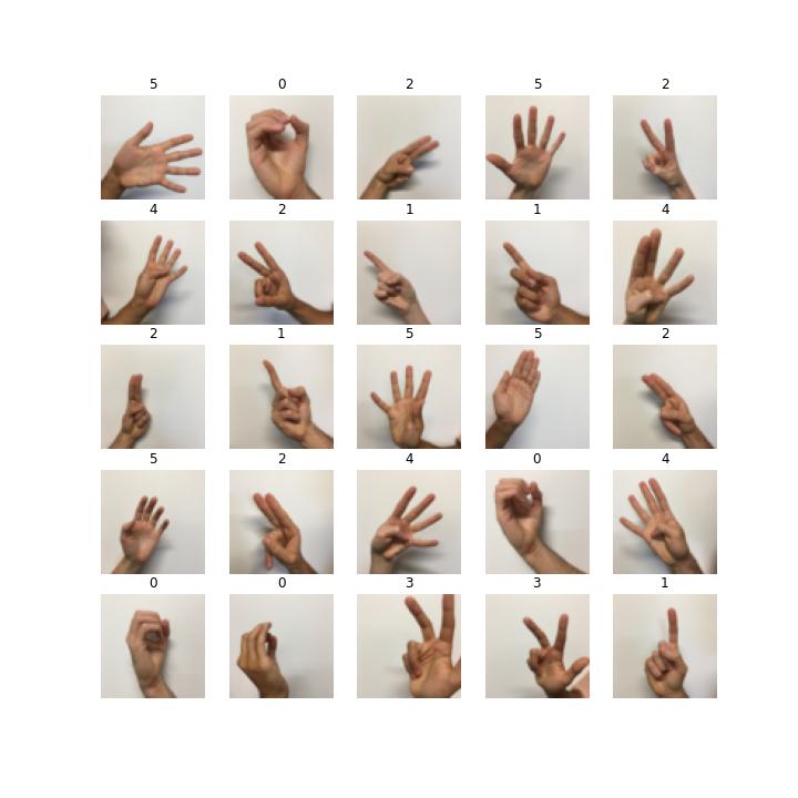
3-Layered NN with Batch Gradient Descent and without Regularization
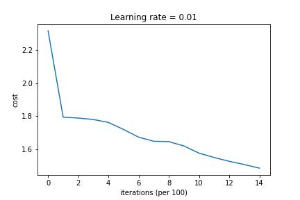
3-Layered NN with Batch Gradient Descent and L2 Regularization
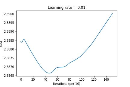
3-Layered NN with Mini-Batch Gradient Descent and L2 Regularization
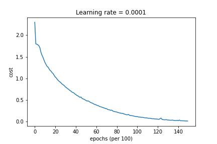
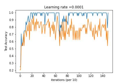
3-Layered NN with Mini-Batch Gradient Descent, Adam Decay and Learning Rate Decay on every iteration

3-Layered NN with Mini-Batch Gradient Descent, Adam Decay and Fixed Interval Scheduling
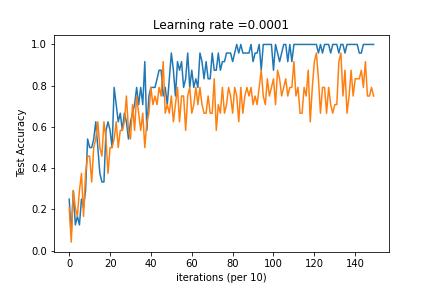
Model multi-classification problem using Tensorflow
